Transient Simulation
The effects of heat storage are not considered using time-independent calculation. Though it has been demonstrated in several studies, how strong heat storage can influence heat transfer (Link Artikel Krakau / Berlin).
AnTherm's ® transient option now allows a simple and physically sound solution to this problem: Just the additional input of the mass density (rho) and the specific heat capacity (c) in the material definition allows transient simulation of already created - or, of course, newly created models. Errors arosen in the neglect of heat storage effects show up most clearly in massive constructions.
For this reason, a 2D edge of a 80 cm thick solid brick masonry should be modeled in a first step of this tutorial and it’s heat flows are calculated.
As a further and more complex example the 3D corner of a foundation slab with exterior walls and spacious adjoining soil is investigated in a second step. In this second example it is demonstrated how the frost line can be found in the ground using the dynamically calculated model.
The chosen investigation period depends on the question to be answered. For this tutorial, the first model is analyzed over the course of a day - for example, a hot summer day. In order to recognize the long-term memory effects of the soil, a one year period was chosen for the second example.
Note: The installed examples can be directly opened with the menu program: Help-> Sample Loading.
> Start with "The objects to be examined"...
The objects to be examined
2D wall edge
The model of a 80 cm thick solid brick masonry (wall edge) with both sides plastered surfaces has to be created.
Overall the wall structure is 84.0 cm thick and consists of (seen from outside):
| 2.5 cm | Exterior plaster |
| 80.0 cm | Solid brick |
| 1.5 cm | Interior plaster |
According to EN ISO 10211 (ÖNorm EN ISO 10211, 2007) the calculation model - a horizontal section through the edge - is bounded by adiabatic layers at a distance of 2.52 m from the edge, measured on the inside.

Fig. AnTherm modeling of solid brick wall edge - 2D Elements window
3D corner foundation slab
In most cases calculating earth-bounding components requires a three-dimensional modeling. Two-or even one-dimensional calculation models can not meet the demands of highly accurate predictability. On the other side, wide areas around the building are affected by the heat flow from the inside. For this reason, the heat storage capacity of the soil plays a very important role. Consequentely the calculation must be time-dependent (transient).
The corner of a foundation slab of a building in passive house standard is going tob e examined.
The corresponding outer wall should be modeled to a height of one meter, as well. The basic system consists of a 20 cm thick reinforced concrete foundation slab, which rests on 20cm extruded polystyrene foam (XPS). The outer wall is a wood stud wall, filled with glass wool insulation - inside with a layer of plasterboard installation completion, outside a 20cm layer of EPS or XPS.
The wall structure is 46 cm thick and consists of (seen from outside):
| 0.3 cm | Organically Bound Plaster |
| 0.3 cm | Plaster |
| 20.0 cm | EPS-F |
| 1.6 cm | Chip board P5 |
| 16.0 cm | Wooden beam |
| inbetween Thermal insulation WLG040 | |
| 1.6 cm | Chip board P4 |
| 5.0 cm | Wood Soft Fibre Board WF043 |
| 1.25 cm | Gypsum fibre board |
The floor structure (base plate) is 57 cm thick, and is composed of (seen from outside):
| 20.0 cm | XPS |
| 20.0 cm | Reinforced conrete-base |
| 10.0 cm | EPS-F |
| 6.0 cm | Cement screed |
| 1.0 cm | Timber planking |
Detail Plans were provided by the company Wolf Haus Austria.
Fig. 2D detail - base slab connecting to external wall (© Wolf Haus Austria)
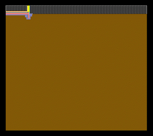
Fig. AnTherm modeling of the foundation slab, exterior walls and surrounding soil - 2D Elements window
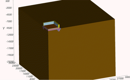
Fig. AnTherm modeling of the foundation slab, exterior walls and surrounding soil - 3D Elements window
Creating the Model
The creation of 2D and 3D models and their transient investigation has already been described in detail in the tutorials "Two-dimensional investigation" and "Three-dimensional investigation". Exactly the same way the models for the transient simulation are created. Sole difference: in the material definition the mass density (rho) and the specific heat capacity (c) must be specified in addition.
Since the typical modeling is already known, the preparation of the sample models is explained only mentioning the most important steps - more attention should be paid to the transient simulation.
2D wall edge
In the main menu choose: File → New #8594; 2D project.
In the "Description" window enter an adequate description of the current project, for example:
| TUTORIAL – Transient simulation: 2D wall edge, 80cm solid brick masonry |
In a first step, it is desirable to specify the building materials. Select View #8594; Data Input and Entry #8594; Materials und Surfaces to show up the desired window.
By clicking the right mouse button onto the materials window you can show the context menu and select "New" or alternatively press the "New" button. A new Material Box appears and in the Material Editor input fields are available.
Press TAB to move the cursor to the name field of the material box.
Enter "Exterior plaster" and TAB to get to the λ (lambda) input field.
Enter 0.8 and TAB to move foreward to the ρ (rho) input field.
Enter 1800 and jump to c-field using TAB.
Type the value 1.3.
In the material list select again "New" from the context menu. You can add two more "blank" material boxes.
Now select the empty building materials and complete the missing data like in the following table:
| Name of building material | λ (Lambda) | ρ (Rho) | c |
| Exterior plaster | 0.8 | 1800 | 1.3 |
| Interior plaster | 0.7 | 1600 | 1 |
| Solid brick | 0,76 | 1700 | 1 |
The colors of the building materials can be adjusted at will.
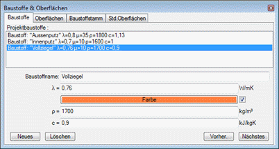
Fig.: Required materials to create the 2D wall edge model - Building Materials window.
Note: With the additional declaration of the mass density ρ and specific heat capacity c you have already met all the requirements to perform a transient simulation.
Make sure that the element input windows are opened. At least "Elements 2D" and "Element Browser" windows should be visible. If not opened, go to the View menu and select View → Primary input window.
The first element inserted should act as the exterior (room). In the Element Browser window, press the „New“ button. The item editor window will appear and a new, empty element is visible in the Element Browser list.
The size of element 1 has to comprise the whole extension of the Model with:
| X_1: | -75 |
| X_2: | 3360 |
| Y_1: | -75 |
| Y_2: | 3360 |
| Type: | Space box |
| Surface description: | outside |
| Rs: | 0.04 |
| Space name: | 0 |
- Begin the entry with coordinates -75 for X1
- Then press the
key to move to the input field X2 - Enter 3360 for X2 and TAB to the next field, which is Y1.
- Enter -75 for Y1 and TAB to Y2
- Enter 3360 for Y2 and confirm again with the TAB key.
- Jump with
to the field surface desription and enter „outside“ - Jump with
to field Rs and enter 0.4 - Jump with
to field room name and enter 0 and confirm the input key
Click the button "Customize" at the upper left of the window „Elemente2D“ to display the model in the overall view.
By using the possibility of the superposed material layers – in which AnTherm only accepts the uppermost lying as valid - the model can be created quickly and easily.
We now operate from the outside to the inside: The next element to be applied is the external plaster:
| X_1: | 0 |
| X_2: | 3360 |
| Y_1: | 0 |
| Y_2: | 3360 |
| Type: | material box |
| Name of material: | Auswahl durch Oberflächenfenster→Außeputz |
Selection through Surface Window→ exterior plasterIn the Element Browser window, press the „New“ button again. Enter the following coordinates listed in the element window and confirm each entry by pressing the TAB key.
Once the "Element Type" field has focus, use the arrow keys to select "material box" as Type. By clicking on the Load button aside you can choose the building material "Exterior plaster" by double clicking in the Surface Window and the material data is applied automatically.
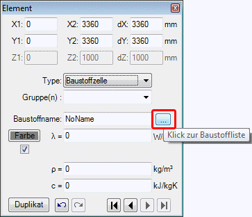
Fig. assigning of material to a material box in the element editor window
The other items have to be entered in the same way:
| X_1: | 25 |
| X_2: | 3360 |
| Y_1: | 25 |
| Y_2: | 3360 |
| Type: | material box |
| Name of building material: | selection through Surface window→solid brick |
| X_1: | 825 |
| X_2: | 3360 |
| Y_1: | 825 |
| Y_2: | 3360 |
| Type: | material box |
| Name of building material: | selection through Surface window→interior plaster |
| X_1: | 840 |
| X_2: | 3360 |
| Y_1: | 840 |
| Y_2: | 3360 |
| Type: | space box |
| Surface description: | inside |
| Rs: | 0,13 |
| Space Mname: | 1 |
Thus, the input of the two-dimensional model is completed.
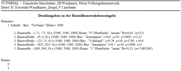
To check the input, select View → Data Entry → Entry report and check the details in the report:
3D corner foundation slab
The three-dimensional, transient calculation of the temperature distribution in general requires the modeling of the entire base plate including very large regions of the soil surrounding the building. The relevant requirements of EN ISO 10211 have to be met.
However, in the case of a rectangular building, the calculation model can be simplified without loss of accuracy according to the following sketch.
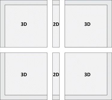
Fig. Distribution of foundation slab without loosing accuracy
For the investigation one of the 4 equal corner pieces is used.
The basic concept of 3D modeling in AnTherm has already been brought closer in the tutorial "Three-dimensional investigation". The following is a rough description of how the 3D model is created; a step by step guide would be too much information for this tutorial. The finished model again can be opened directly under: menu Help → Example Loading.
As an alternative to modeling directly in AnTherm, in this case the 2D vertical section of the base slab and the outer wall has been created in a CAD program. The CAD file in DXF format is then imported into AnTherm. If you do not using a CAD software, alternatively the Dxf file can be imported from the program directory Antherm/examples/.
It is up to you, if you create a new 3D project, or if you initially generate a 2D project, and then convert the 2D project for further processing into a 3D project. This way you'll have a finished 2D project available for possible future investigations of the 2D vertical section.
So create a new 2D project. Import the CAD vertical section through the main menu File → Import →aCad DXF. Select the file from the Antherm_Fundamentplatte.dxf from Antherm/examples directory program. The material boxes were drawn as poly-lines und put on appropriate layers. When importing, it is advisable to name the materials same like the layer name. Following the illustration of the dxf import:
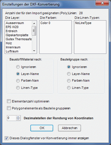
Fig. DXF import of the base slab - Import by layer name.
After confirming with "Ok", the geometry of the 2D vertical section is imported into AntTerm.
Also the rooms have already been drawn in the CAD (Dxf). They have to be declared as space boxes (Type) with appropriate parameters (see Example 2D wall edge) in the element window.
The next step is the entry of building materials. Update the materials according to the following list:
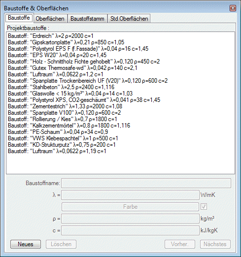
Fig.: Required materials for the model base slab
You now already can do a transient two-dimensional calculation. However, this tutorial explains the transient simulation of a 3D model, so you have to save the 2D project for any subsequent investigation and then convert it into a 3D model. Use: File → Convert → Layers 3D Project. Due to the complexity of the selected model it results in a large number of extruded 2D layers in order to complete the 3D model:

Each layer can be duplicated from the preceding, and the changes required can be made. You can also skip this step by loading the completed model from the samples folder. The list of layers is shown in the following figure:
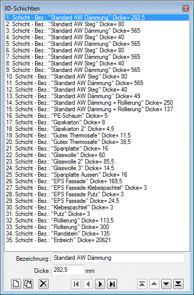
Fig. 3D layers
Obtain main results – evaluation
After the model was completed, the transient simulation can be started. Select in the main menu "Results ...".
You will be prompted to save the project data, for specifying fine grid and solver parameters and due tu using the non-stationary extension also to enter the parameter for the transient simulation. The preset default parameters for the fine grid and the solver are suitable for most cases , as well as this tutorial-example.
In order to perform the transient calculation, the option "Compute Transient Periodic Solution" in the "control parameters of the transient, periodic, harmonic calculation" must be activated. The control parameters for the transient simulation must be defined depending on the question. A step by step guide to the two models follows in the subsections "2D wall edge" and "3D corner foundation slab", but for now information on the general process:
After the specification of the control parameters, the calculation is started by confirming with "OK" in the "SolverParameter" window.
After successful calculation the Coupling Coefficient Report is presented and the calculation independent boundary conditions can be determined arbitrarily.
At the stationary investigation simply the temperature of the modeled spaces (at an exact point in time) was required as boundary condition - due to the time-independence. If one wants to examine a building-component over a period of time, it is also necessary to specify the boundary conditions variable in time.
AnTherm offers some very simple ways for the user to define the periodically changing boundary conditions.
For example, as values on points of equal distance (regular points), as means to uniformly or arbitrarily long intervals (Regular Means, Irregular Means), or as step values (switching) or as irregular time intervals (Irregular Steps). Furthermore, any periodic distribution can be specified as a series of Fourier coefficients.
Note: the modeling of the periodic boundary conditions is not only limited to the temperature but is also possible for voluminous heat-sources or -sinks.
2D wall edge
After the item "Results ..." was selected in the main menu, the settings for the transient simulation must be determined in the "SolverParameter" window. For the analysis of the 2D wall edge on a summer day the option "day (24 hours)" must be activated.
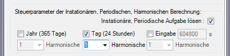
To keep the calculation time very short and, since the course of the outside temperature anyway - as described hereinafter - follows a sine curve, the selection of only one harmonic for this calculation is sufficient. For other investigation cases with other types of boundary conditions, it is advisable, however, in favor of the accuracy of the calculation to use a higher number of harmonics.
By confirming with "Ok", the calculation is performed. This may take some time depending on the model and number of harmonics.
Once the construction of the basis solutions has been successfully completed, the Coupling Coefficients are created and displayed in the thermal conductance report. Also the window of the boundary conditions is shown. How the input of periodic boundary conditions works will follow soon, but for now the report of the thermal conductances:
The Coupling Coefficients Report contains a set of values that are necessary to exactly describe the construction. The Coupling Coefficients Report is divided into sections by horizontal lines. How can these values of each section be understood?
The first section contains the thermal conductance of the zeroth harmonic. This is the already known stationary conductance. In the stationary case, the conductances of the investigated wall edge 2D of space 0 (external space) is toward the space 1 (space), and vice versa 4.27 W / (mK). However, in order to describe the dynamic behavior of the structure, it requires the additional thermal harmonic conductances. In this case, a harmonic has been selected for the calculation, so that a further range of values, separated by the horizontal line, is added. So in this section you will find the harmonic conductance for the first harmonic (period 86400sec, that is one day). Would there have been specified several harmonics beforehand, for each harmonic a section would get added for the thermal conductance with its respective period length.
It is notable that in contrast to the stationary - the harmonic conductance is now representing complex numbers - a real part and an imaginary part. For a better understanding, the conductance values are presented in a second matrix using the absolute value (amplitude) and the argument (phase shift). Therefore, each section of the harmonic conductance contains two matrices / tables. This output allows, for example, the easy reading of the external harmonic conductance (from outside to inside) and the phase shift of the construction. In contrast to the steady-state case the diagonal elements are very important and can be used for calculating the effective thermal storage mass.
Note: In this way the area-related harmonic thermal coupling coefficients y (i, j) of EN ISO 13786 can be calculated very convenient.
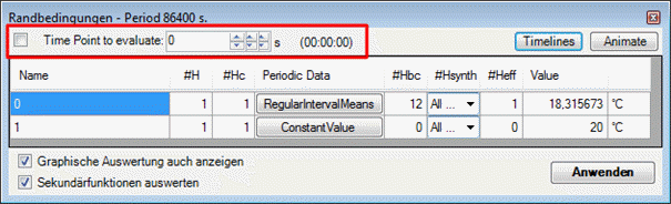
But now let’s go on to the description of the periodic boundary conditions. The following figure shows the window with the overview of the boundary conditions:

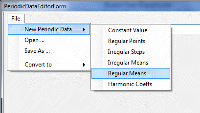
For the 2D wall edge the boundary condition on the outside - in this example, the area 0 - the temperature of a hot summer day can be specified. Click on the button "Constant Value" of the outer space "0". This will open the window to determine the periodic boundary conditions. By default, a constant value (such as in the stationary analysis) is defined. To enter the desired course of the day, choose New Periodic Data → Regular Means.
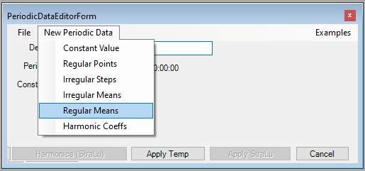
In the following dialog enter a name for the periodic boundary conditions. Mind the period length corresponds to one days (86400sec) and if 24 intervals (24) are specified.
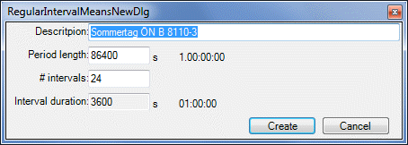
Create the new periodic record by "Create".
The outside air temperature will be determined according to the standard summer day based on ÖNORM B8110-3. In Annex A of the standard the deviation of the daily mean temperature is given over the day, in the following table, the deviation is already summed up to the selected upper limit of the average daily temperature of 23 ° C:
| h | Temperature |
| 00:01 | 18,28 |
| 00:02 | 17,37 |
| 00:03 | 16,63 |
| 00:04 | 16,07 |
| 00:05 | 15,72 |
| 00:06 | 15,76 |
| 00:07 | 17,17 |
| 00:08 | 19,51 |
| 00:09 | 22,04 |
| 00:10 | 24,33 |
| 00:11 | 26,18 |
| 00:12 | 27,58 |
| 00:13 | 28,57 |
| 00:14 | 29,20 |
| 00:15 | 29,55 |
| 00:16 | 29,64 |
| 00:17 | 29,40 |
| 00:18 | 28,70 |
| 00:19 | 27,52 |
| 00:20 | 25,96 |
| 00:21 | 24,19 |
| 00:22 | 22,41 |
| 00:23 | 20,79 |
| 00:24 | 19,41 |
The 24-hour values of the temperature gradient can be easily entered by double-clicking the fields in the Value column of the Periodic Table Data Editor. The input is interactive: When a value is specified, the chart is updated and the values can be checked visually. There is also the possibility of scaling the bars in the chart, by clicking the upper side of a bar and moving simultaneously. But it is recommended having prepared temperature values and using the editable table - for accurate input.
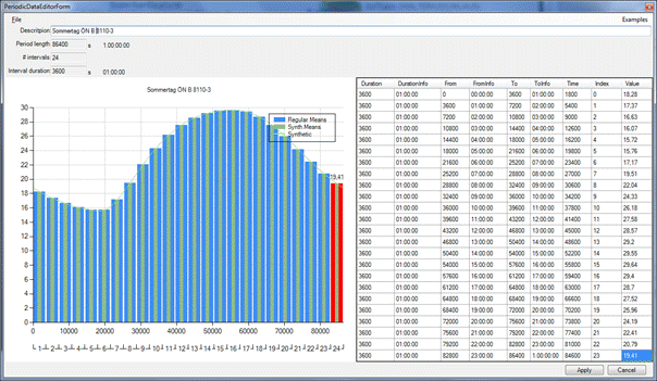
After you have entered the values, save this data under File→Save as… to have the possibility of re-opening it for any future use. Confirm the entry with "Apply".
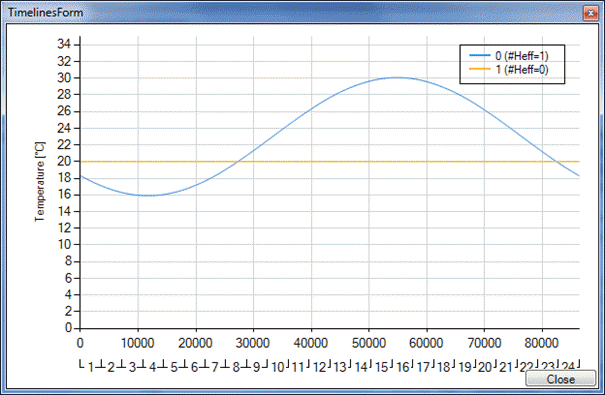
Note: You clearly can see that the course of the temperature of the ÖNorm follows a sine curve. Another type of periodic data entry would have led to similar results: About → File → New → Harmonic Periodic Data Coeffs a new record with the period length of 86400sec and one harmonic could have been created. For the real part of the zeroth Harmonics would have been declared the value 23 (so to speak the daily mean value) and the second harmonic can specify a value of 7 (the oscillation). In order to put the sine curve to the correct position, you have to specify a phase shift (ArgDeg), for example 130°.
You are now passed back to the overview window of the boundary conditions.
Another difference to the overview window of the stationary calculation is the two buttons "Timelines" and "Animate". By clicking on "timelines" a window opens, in which the time courses of the boundary conditions are displayed and can be checked:
The other button "Animate" allows an animation over any period of time to export as a video. This function is only executed when the 3D results window is already opend and a desired display is set - it is discussed in the section on "Graphical Analysis" in more detail.
In the upper left corner you can now select any of the time point of the day. Set the desired time for the examination.
Confirm the set of boundary conditions now by clicking on the Apply button.
After a short waiting period, in which the temperature distribution in the component is calculated, the results appear in the results report.
You can now also perform graphical analysis for the specified time point - and without having to perform the calculation again, select a different time point in the window and click "Apply" for further investigation.
3D edge foundation slab
After the item "Results ..." was selected in the main menu, the settings for the transient simulation must be determined in the "SolverParameter" window. For the Analysis of the 3D foundation slab with surrounding soil over the course of the year the "year (365 days)" checkbox must be activated.
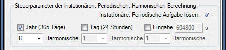
For the outdoor temperatures 12 months average-temperature-values are given. To represent this accurately, it is recommended to set a higher number of harmonics (6).
By confirming with "Ok", the calculation is performed. Due to the complexity of the model and the number of 6 harmonics , the calculation may take some time depending on the hardware configuration.
Once the construction of the basis solutions has been successfully completed, the coupling coefficients are created and displayed in the report of the thermal conductances. Also the window of the boundary conditions is shown. How the input of periodic boundary conditions works will follow soon, but for now the report of the thermal conductances
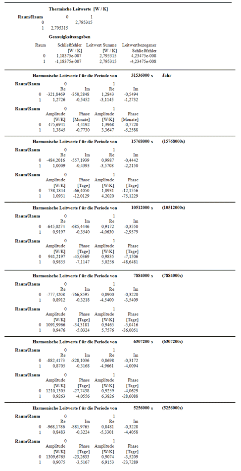
In the first section of the Coupling Coefficient Report you can see the stationary conductances, in subsequent sections then the conductance of each of the six harmonics. The detailed description of the individual values was already shown in the example "2D wall edge." You can find additional information in the description of the Coupling Coefficient Report.
But now let’s go on to the description of the periodic boundary conditions. The following figure shows the window with the overview of the boundary conditions:
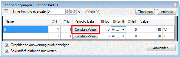
For the 3D foundation slab the boundary condition on the outside - in this example, the area 0 – the course of the temperature over the year is given by monthly mean temperatures (Krakow). Click on the button "Constant Value" of the outer space "0". This will open the window to determine the periodic boundary conditions. By default, a constant value (such as in the stationary test) is defined. To enter the desired course of the year, choose File → New → Regular Periodic Data Means.
Enter in the following dialog a name for the periodic boundary conditions and ensure to care if the period length is one year (31536000 seconds) and if 12 intervals (12 months) are specified.
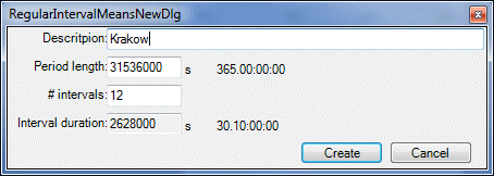
Create the new periodic record by "Create".
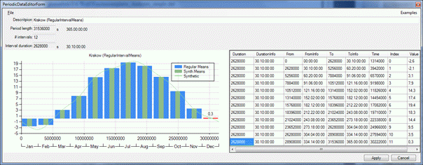
The outside air temperature will be determined according to the monthly mean temperatures of Krakow. The following table shows the monthly mean temperatures:
| Month | Temperature |
| Jan | -2,6 |
| Feb | -2,1 |
| Mar | 3,1 |
| Apr | 7,9 |
| May | 14,3 |
| Jun | 17,4 |
| Jul | 19,4 |
| Aug | 18,3 |
| Sep | 14,4 |
| Oct | 9,5 |
| Nov | 3,5 |
| Dec | 0,3 |
The 12 monthly mean values of the temperature gradient can be easily entered by double-clicking the fields in the Value column of the Periodic Table Data Editor. The input is interactive: When a value is specified, the chart is updated and the values can be checked visually. There is also the possibility of scaling the bars in the chart, by clicking the upper side of a bar and moving simultaneously. But it is recommended having prepared temperature values and using the editable table - for accurate input.
After you have entered the values, save this data under File → save as… to have the possibility to reopen it again for any future use. Confirm the entry with "Apply".
You are now passed back to the overview window of the boundary conditions.
As explained in the „2D wall edge-example“, you can again check profiles of the boundary conditions by clicking on „Timelines“
The button "Animate" allows an animation over any period of time to export as a video. This function is only executed when the 3D results window is already opend and a desired display is set.
Now a date for the investigation can be set, or it may also be an animation created over the course of the year. This will be explained step by step in the „Graphical Analysis“.
Confirm the set of boundary conditions now by clicking on the Apply button.
After a short waiting period, in which the temperature distribution in the component is calculated, results appear in the results report.
Graphic evaluations
In the transient simulation, the time is added as an additional dimension. It can now be analyzed at any arbitrary point in time (in seconds) of the selected period in the usual stationary manner - the graphical analysis is then carried out in the same way as in the stationary calculation - after determining the time point in the boundary conditions window. This has already been described in detail and can be read in the tutorials "Two-dimensional investigation" or "Three-dimensional investigation".
Now there is also the possibility, to represent the temperature distribution on a section plane for several successive time points at certain intervals in the manner of a slide show. This type of visualization gives the user a feeling of the effects of heat transfer and heat storage in the component over a specified time period.
In the following section an animation over the course of the temperature distribution in the two models (2D and 3D edge wall foundation slab) is created.
2D Wall Edge
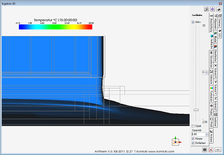
After applying the boundary conditions choose an appropriate view in the 3D results window such as the following illustration shows - of course you can choose any other representations (isolines, heat flow lines, etc.), as well. If you we want to visualize the color bar with labeling, pay attention to set a "Fixed values range" in the tab "color bar" in the Results 3D window – otherwise there would be a dynamic range of values for any timepoint of the animation (which is not appropriate for the comparison). You can also customize the range of values to get a more suitable result during the course of the temperatures over time. You could set the range between 16 ° C and 30 ° C.
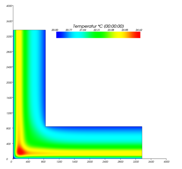
Fig. 3D results window of the 2D wall edge at time 0 with dynamic range of values for the color bar
Since the conditions for the export of animation are now done, you can switch to the Boundary Conditions window:
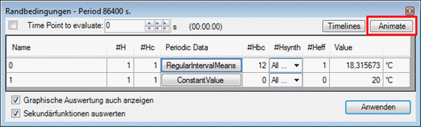
Fig. Bounding conditions window with the Animate button to create animations
Click the "Animate" button to create an animation. Subsequently, a window opens the settings for the animation:
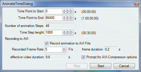
Fig. Animate dialog for the settings of the animation
In the "Animate" dialog the period is set by default, but can be changed on request. For this demonstration, the entire period was retained - thus the entire course of the day is the correct duration. The "Time Step Length" - the interval until the next frame analysis - has been set here at 1800 seconds, which is every 30 minutes to represent the change of the temperature field in the animation.
Activate the option "Record to AVI animation file" to export the animation as a video file. By clicking "Start" a dialog will open that determines where you want to save the animation. Enter a suitable name and confirm with "Save". Before the animation starts (and the video file is written), a last dialog with settings for the video compression pops up. You can use the default settings and skip it. After the animation is finished the video file is created as well. You can play in any video player.
In this 2D example you can clearly see a "heat bubble" in the corner. Only the transient simulation allows to detect such effects and to analyze it.
3D Corner foundation slab
After Clicking „Apply“ in the Boundary Conditions Window the 3D-Result Window ist beeing opened besides the Result Report. You now can analyze the 3D model at the timepoint (stated in sec. – standard timepoint = 0) specified in the boundary conditions window.
Same like before in the 2D example, it is also possible to create an animation of the thermal behaviour of the 3D slab over the course of the year. For this have a look at the 2D Wall-Edge example and change the parameters for your needs. For the animation settings you need to know the end of the animation, which is 31536000. The timestep can be set to 86400 seconds – so each day results are part of the animation
Determining the frost line
The question about the frost line in the soil plays an important role. Due to the ensuring of frost-free foundations, a long-term average (temperature) calculation can not be used directly. To get correct results, extreme winter outside climatic conditions must be applied. In this case the extreme winter temperatures of a 50-year time series of ambient air temperature values between the years 1960 and 2009, measured at the meteorological station of Vienna, Hohewarte were extracted. The only year (1996) were the monthly mean values for December, January and February were below the freezing temperature was selected and set as basis of the simulation.
For the existing 3D model (the base slab), the frost line is to be determined now. For this purpose, the periodic boundary conditions on the outer side (area 0) must be changed.
As well as previously done with the monthly mean temperatures create a periodic record with 12 intervals and a period of one year (31536000 seconds). Now do not enter the monthly mean temperatures of the long-term annual cycle of the outside air temperature (Krakow) as before, but the extreme values of 1996 (Hohewarte, Vienna):
| Month | Temperature |
| Jan | -2,71 |
| Feb | -2,45 |
| Mar | 2,07 |
| Apr | 10,09 |
| May | 15,49 |
| Jun | 19,04 |
| Jul | 19,4 |
| Aug | 18,52 |
| Sep | 18,93 |
| Oct | 12,31 |
| Nov | 7,09 |
| Dec | -2,23 |
Basic principle to check frost free conditions of the foundation in the current version of AnTherm ®:
- in a 2D case to find out the lowest position of the 0 ° C isotherm in the ground and to check whether this ia below the foundation construction.
- In the 3D you need to use the the 0 ° C iso-surface for analysis.
An easy way how to check whether the foundation over the entire course of the year remains frost-free is introduced now:
First, one has to find out the timepoint of the lowest position of the 0 ° C iso-surface. The 3D foundation slab corner already was calculated transient using for example 6 harmonics for the course of the year and as a boundary condition the extreme values of 1996 have already been assigned for the exterior space. The coldest month is January as shown in the table above. It is known that the heat storage of the soil causes phase shifts - depending on the material properties of the soil – this phase shift can easily be several weeks. Visually you can quickly find out the day with the deepest isotherm by watching the animation, for example, over the first three months of the year. Once you have specified the day, you can check the frost-free conditions of the foundation in further steps.
As a preset for the animation the color bar should be positioned clearly visible in the 3D viewing window because the current timepoint is displayed within the header of the bar. Start the the 3D viewing window before creating the animation by setting, for example, the 15th day as time point in the boundary conditions window. Then click on the button "Apply".
For the animation it is also important to assign a fixed value range to the color bar and as well as for the isolines (2D) or isosurfaces (3D). For this example choose as lower value the lowest outside temperature of -2.71 ° C and 20 ° C as the upper value for the color bar. If you want to visualize isolines fix the range of values here, as well. Since the 0 ° C iso-surface should be displayed for this 3D example, set a fixed range of the values of the "iso-surface" tab of the 3D viewing window with upper and lower limit of 0 ° C. Now you can already see the representation of the isosurface. It may be necessary to adjust the visibility - turn off the opacity and specify a visibility of 0.9 for example. The contours of the model are visible in a better way.
Here, the surface representation has been disabled in the corresponding tab to make the iso-surface clearly visible. You may well recognize the decrease in the 0 ° C iso-surface in the corner of the foundation. So you can see, in these cases a 3D analysis is very important.
If the above settings for the 3D viewing window were applied, you can start with the animation settings by pressing the Animate button in the Boundary Conditions window. In this case you could set the first 60 days of the year as animation duration (start: 0 seconds end: 5.184 million seconds). As time step specify a day (86400 seconds). You can then start the animation and for later use also have the possibility of recording it. In the next step one can observe if the frost line (0 ° C iso-surface) is below the foundation or not. You can easily find the day of the lowest position of the iso-surface. Exactly this day you can then examine in more detail in a further analysis. Thus, for example, you can find out the the exact temperature at any point by using the function of sample points.
This investigation has shown that the structure remains permanently frost free (at the lowest point of the foundation) even in the corner in an extremely cold year.