Boundary Conditions window

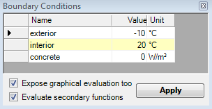The window Boundary Conditions enlists all spaces of  which the user sets temperatures and all power sources of which power density can be entered (the boundary conditions). For dynamic, transient problem solution the window mutates to allow input of time dependant quantities.

Temperatures of spaces are initially preset to standard values:

• first space in the list (sorted alphabetically) is set to airspace temperature of -10°C
• all other spaces are set to the temperature of +20°C.

Remark: These standard values can be changed within application settings.

Spaces are enlisted alphabetically. Knowing this, by consequently naming spaces you can target proper automatic assignment of preset values.:

• Exterior precedes Interior
• Space 00 precedes Space 03 and Space 10
• Space 11 precedes Space 1.

If the component contains power sources (heat sources or sinks) also, their names will be offered here for the input of their respective power density [W/m³]. Initially power sources are set to have no power (equal 0 W/m³).

Remark: If there is solution of vapour calculation available too, the input of relative humidity of air space, required for vapour evaluations of partial pressure, is also offered in additional dedicated column:

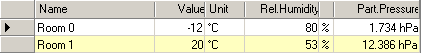
Relative humidity of air spaces is initially preset as follows:

• first space is assigned the relative air humidity of 80%
• all further spaces are assigned relative air humidity of 53%.

Remark: These standard values can be changed within application settings.
 

Name	Name of the space or power source (not editable)
Value	The value of the boundary condition of specific space (temperature °C) or power source (power density W/m3).
Unit	Unit of the value of that specific boundary condition (not editable)
Rel. Humidity	Relative air humidity in percent
Part. Pressure	Partial pressure of vapour (in hPa) resulting from the temperature and relative humidity values entered (not editable)
Expose graphical evaluation too	If checked here, the graphical evaluation (Results 3D window) will be started after boundary conditions are applied. If this setting is turned off the graphical evaluation (if not open yet) will not be executed automatically. See also Application settings.
Evaluate secondary functions	If checked here, secondary functions (like heat flux, relative surface humidity, etc.) will be calculated for graphical evaluation. If turned off (unchecked) only temperature field will be calculated for Results 3D evaluations. This saves significantly time needed for calculation and reduces memory demand during evaluation. See also Application settings
Apply	Confirms data entered in this window end initiates the superposition followed by various evaluations.

You confirm the data entered by pressing the button Apply. Boundary conditions will be applied onto basic solutions (g-values). If calculation of basic solutions is also required it will be automatically initiated also.

MULTICORE-option: Speeding up computationally intensive jobs by distributing them on multiple processors or processor cores for parallel execution is only possible with an active MULTICORE-Option of the program.

Remark: The button "Apply" will blink if there is new solution set available from the solver, but the data entered in this window has not been applied yet to the new solution set.
Remark: The button "Apply" is shown disabled if one or more basic solutions have not been calculated (solved) yet, i.e. they are missing.

The temperature distribution with the construction results from the superposition of respective basic solutions each multiplied by its boundary condition. Results are presented as text reports ready for printing or to be saved as Adobe PDF, MS.Word or MS-Excel files.
The distribution of temperature and further secondary functions is further used in various graphical evaluations.

Templates of Boundary conditions are saved to the project file when the project is saved.

Remark: All BCs will be merged by their Names into the projects BC-Template upon apply. This will retain BCs even when spaces or power source are renamed or removed from the project. By that the BCs of other projects can be merged and saved - even such with names which are not yet (or no more) available if the current project.

Important: To retain the values of boundary conditions between program executions the project must be explicitly saved (project data is not saved automatically when boundary conditions are applied!).

Remark: You will need the value of power density W/m³ to properly enter the boundary condition specific to power sources. For verification purposes you will find the total volume of each power source within Modelling Report. Within Results Report, in addition to the value of respective power densities, you will also find the overall power of each power source.

VAPOUR-option: Analysis of multidimensional vapour diffusion is only possible with an active VAPOUR-Option of the program..

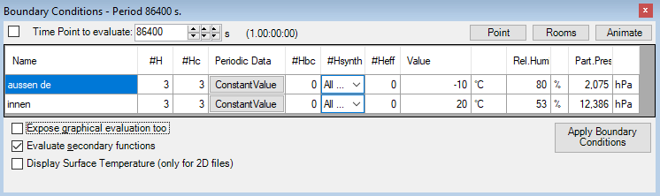
Transient Boundary Conditions (periodic, harmonic)

For the purpose of dynamic, transient problem (subject to the TRANSIENT-Option) the boundary conditions window mutates to input of time dependant quantities.

TRANSIENT-option: Solving and evaluating time dependant dynamic, periodic problems when heat capacity effects are concerned is only possible with an active TRANSIENT-Option of the program.

The transient boundary conditions are provided as sets of harmonic Fourier coefficients created for respective periodic data (these are managed in Periodic / Harmonic Data Editor) for each and any Main Period of the transient problem (as selected in Solver parameter form).

Boundary conditions are kept distinct of each solution period and also saved to the project file when the project is saved. Important: To retain the values of boundary conditions lately applied the project must be explicitly saved (project data is not saved automatically when boundary conditions are applied!).

Remark: All BCs will be merged for each Period (including MainPeriod=0 - steady state) by their Names into the projects BC-Template upon apply. This will retain BCs even when spaces or power source are renamed or removed from the project. By that the BCs of other projects can be merged and saved - even such with periods and names which are not yet (or no more) available if the current project.

Main Period (title-bar)	The Boundary Conditions window title bar displays the Maine Period of the currently evaluation transient, periodic problem (as selected in Solver parameter form).
Time Point to evaluate	Some evaluation time point T within the Main Period of the solution. If checked the change to the time point is immediately applied together with boundary conditions and reflected in evaluation windows (Results report, Results 3D window) once these are open.
#H	Number of harmonics solved (harmonic solutions) for the selected Period and available to further evaluation
#Hc	Number of continuous harmonics solved for the selected Period and available to further evaluation
Periodic Data	Periodic boundary conditions data managed in Periodic / Harmonic Data Editor By default the Constant Value Periodic data will be initially set respectively to the steady state boundary condition.
#Hbc	Number of harmonics available from Fourier Analysis out of periodic boundary conditions data (managed in Periodic / Harmonic Data Editor) available to further synthesis and evaluation
#Hsynth	Number of harmonics chosen for use in harmonic Fourier Synthesis out of those available from periodic boundary conditions data (#Hbc) The highest number of harmonics used during synthesis (#Hsynth) results from the smallest count of harmonics within the base solution and out of the respective boundary condition and can be further reduced (-1 - all available). Remark: Evaluating in TRANSIENT mode with only 0-th harmonic or only Constant Boundary Conditions is identical to Steady State results (regardless of HARMONIC or TRANSIENT license feature).
#Heff	Effective number of harmonics used in harmonic Fourier Synthesis out of those available from periodic boundary conditions data (#Hbc) and those available from the solution set (#H).
Value	Synthetic boundary condition value at the evaluation time point T
Point	Opens the Point window displaying the synthetic timeline of a chosen point.
Timelines	Opens Timelines window displaying timelines of synthetic boundary conditions applied.
Animate	Displays the Animate Time Dialog used to define temporal animation of transient evaluation by automating changes to the evaluation time point T.

Time Point to Evaluate: provided existence of periodic boundary conditions on can set the evaluation time point (within the main period)

Remark: During graphical evaluation the time point information will be displayed in the title of the colour bar.

For the evaluation the harmonic base solutions are combined with the respective harmonic coefficients of the boundary condition the belong to (complex linear combination). The resulting distribution harmonic coefficients it then passed for Fourier synthesis for specific evaluation time point T.

Remark: Provided that the periodic boundary conditions did not change, only synthesis for new time point must be executed.

Remark: Evaluating in TRANSIENT mode with only 0-th harmonic or only Constant Boundary Conditions is identical to Steady State results (regardless of HARMONIC or TRANSIENT license feature).

MULTICORE-option: Speeding up computationally intensive jobs by distributing them on multiple processors or processor cores for parallel execution is only possible with an active MULTICORE-Option of the program.

Remark: The input of relative air humidity (when vapour diffusion problem has been solved too) are sill constant (steady state) and independent of air temperatures. Only the partial pressure will be recalculated for respective, evaluation time point dependant, air temperature.

See also: Element Editor, Element types, Evaluations and Results, Standard Boundary Conditions, Periodic / Harmonic Data Editor, Animate Time Dialog,  Timelines Window